Most of the objects we have learned about so far, are so-called dataflow objects (at least Miller Puckette, the inventor of Pd, put them in this category). Besides these, Pd also has a lot of audio objects. These can easily be distinguished by the ~ (tilde) after their name. The ~looks like a little sound wave. Objects with a ~ deal with everything related to (sound) signals, so that’s easy to remember. Also, these objects are much faster than dataflow objects. We have already gotten to know some of the audio objects in the last lecture when we played sounds with [readsf~], [*~] and also used [dac~] for playing back sounds. We have also noticed, that the cords which transport audio-signals are much (a bit) thicker than the usual black patch cords we use for sending normal messages.
Setup
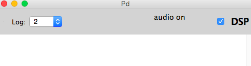
Before starting with sound, let’s have a look if sound processing is switched on. We need a checkbox in the Pd window.
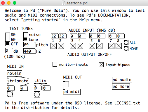
We can easily test if everything is working by choosing Menubar->Media->Test Audio and MIDI…:
If you do not hear the test tones, check the Audio Settings via the Menubar->Media->Audio Settings: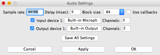
readsf~, dac~
Let’s summarize the objects we already know. Last week we have played back samples using [readsf~].
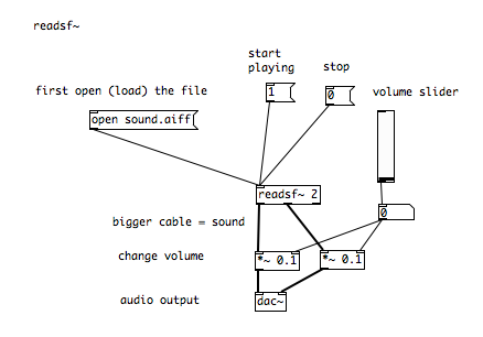
[readsf~] plays audio files from your disk. Just like playing back files, Pd can also record files to your disc. The object you need for that is [writesf~].
writesf~ and adc~
[writesf~] is used to record sound files to your hard disk. The setup we need for recording sound reminds us of the setup to play files. However, instead of using the [dac~] to output audio, we need something to input audio. This is the [adc~], an analogue-digital converter. By default, the left outlet is for the left channel and the right outlet for the right channel. We use only one channel and therefor put a 1 as an argument. We connect it to the input of [writesf~]. Sending the message ‘open filename.wav’ allows us the select a file name (and if we want to, also a path) for the file we will record. Sending a ‘start’ message will start recording, a ’stop′ message will stop it. (0 and 1 do not seem to work!).
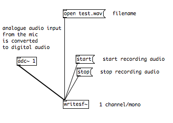
Note, that this results in a mono recording, but we actually record 64 channels at once!
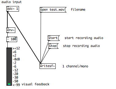
VU meter
We can also add some visual feedback, so we can detect possible problems before listening back to the recording. The VU meter object (Menubar->Put->VU meter) can give us visual feedback about the amplitude of a signal. In order to do so, we also need a [env~] object (which takes a signal and outputs its root mean square amplitude in dB). (Because the [env~] provides us with values from 0 db to 100 db we have to subtract 100 from the values before we can display them in the way that makes sense.)
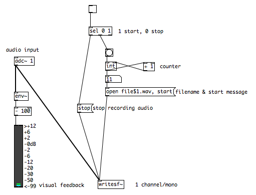
Bonus: Make automatically numbered recordings with one click.
We can use what we have learned so far to make recordings which are started and automatically named with ascending numbers with the switch of just one toggle.
Additionally to record and play back sounds, Max can of course be used to produce sounds. In the following I will give a very quick overview of some options.
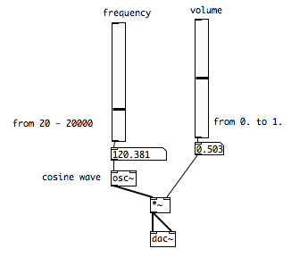
osc~
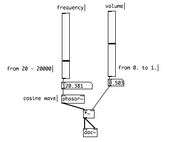
We use [osc~] to generate our first test tone. [osc~] is a oscillator that reads repeatedly through one cycle of a waveform. You’ll learn more about what that is and means in the Sound Space Interaction course. Don’t worry if you don’t know it yet. What matters now is that by default, it puts a cosine wave out (which sounds exactly the same as a sine wave!). The left inlet takes a frequency, so you can produce cosine waves in any frequency. You probably know that when young we can hear approximately between 20 and 20000 Hz (herz) but with getting older, you can hear less high. Let’s make a test to find out how high you still can hear. We can play back the cosine wave just like the audio file on our computer. Again, we use [*~] in combination with a slider to adjust the volume.
phasor~
We have used [osc~] to generate a cosine wave. [phasor~] is a sawtooth wave generator. It takes a frequency into its left inlet and puts out a sawtooth wave with that frequency. Edwin will tell you much more about the underlying principles. Enjoy some experimenting and compare the audible difference between the previous patch using [osc~] and this one:
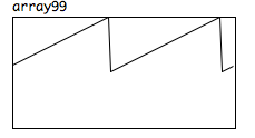
In case you are interested, this is how the phasor-signal looks when it is written into an array:
noise~
[noise~] is another sound generator. However, this one does not take a frequency. That’s because it generates so called white noise. Formulated a bit too simple, just like white light contains all colors at once, white noise contains all frequencies. Wikipedia formulates it like this: the signal contains equal power within a fixed bandwith at any center frequency. Don’t worry if you don’t understand that yet, but please listen to it. If you were asked if this sounds low, high or like a specific note, you should not be fooled. They are all in there.
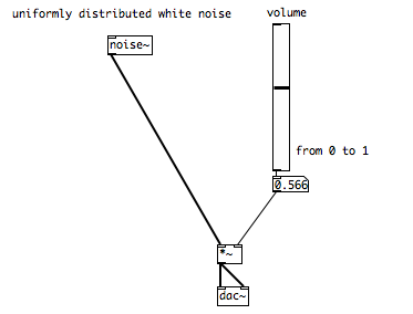
You could use a line object to change the volume to make it sound a bit like waves on the beach.